Trend modeling
This example (from the GMT gallery - EX45) shows how the module trend1d is used to fit the CO2 data set collected from the top of Mauna Loa. This yields the famous Keeling curve.
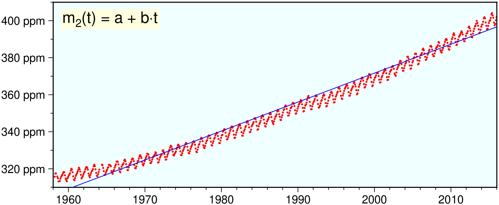
Basic LS (Least Squares) line y = a + bx
using GMT

model = trend1d("@MaunaLoa_CO2.txt", output=:xm, model=(polynome=1,))
plot("@MaunaLoa_CO2.txt", region=(1958,2016,310,410), frame=(axes=:WSen, bg=:azure1),
     xaxis=(annot=:auto, ticks=:auto), yaxis=(annot=:auto, ticks=:auto, suffix=" ppm"),
     marker=:circle, ms=0.05, fill=:red, figsize=(12,5))
plot!(model, pen=(0.5,:blue))
text!(mat2ds("m@-2@-(t) = a + b@~\\327@~t"), font=12, region_justify=:TL,
      offset=(away=true, shift=0.25), fill=:lightyellow, show=true)
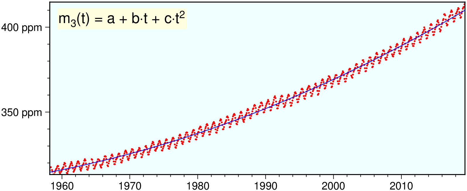
Basic LS line y = a + bx + cx^2
model = trend1d("@MaunaLoa_CO2.txt", output=:xm, model=(polynome=2,))
plot("@MaunaLoa_CO2.txt", frame=:same, ms=0.05, fill=:red, figsize=(12,5))
plot!(model, lt=0.5, lc=:blue)
text!(mat2ds("m@-3@-(t) = a + b@~\\327@~t + c@~\\327@~t@+2@+"), font=12,
      region_justify=:TL, offset=(away=true, shift=0.25), fill=:lightyellow, show=true)
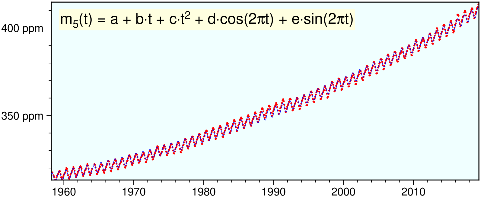
Basic LS line y = a + bx + cx^2 + seasonal change
model = trend1d("@MaunaLoa_CO2.txt", output=:xmr, model=((polynome=2,), (fourier=1, origin=1958, length=1)))
plot("@MaunaLoa_CO2.txt", frame=:same, ms=0.05, fill=:red, figsize=(12,5))
plot!(model, pen=(0.25,:blue))
text!(mat2ds("m@-5@-(t) = a + b@~\\327@~t + c@~\\327@~t@+2@+ + d@~\\327@~cos(2@~p@~t) + e@~\\327@~sin(2@~p@~t)"),
      font=12, region_justify=:TL, offset=(away=true, shift=0.25), fill=:lightyellow, show=true)
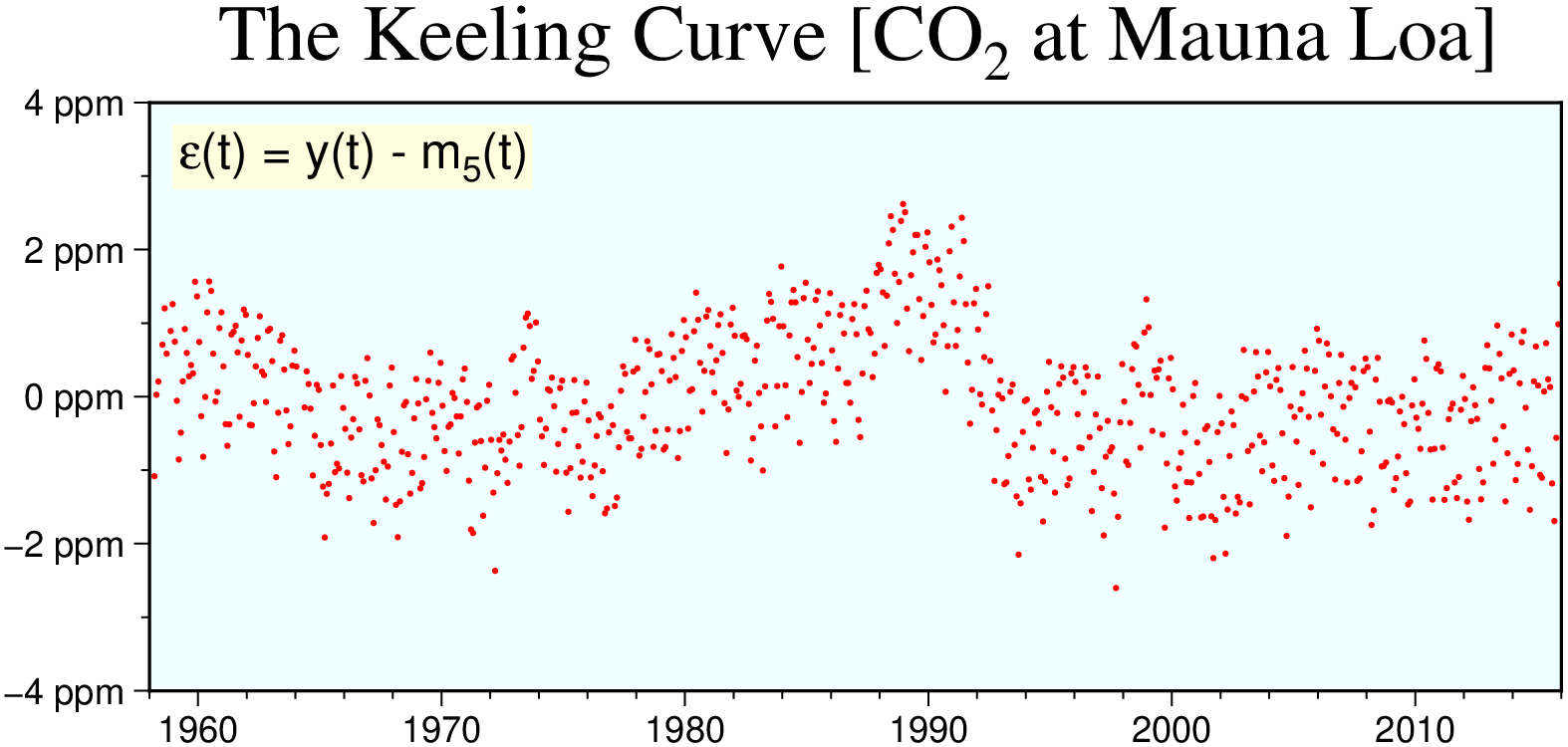
Plot residuals of last model
plot(model, region=(1958,2016,-4,4), frame=(axes=:WSen, bg=:azure1,
      title="The Keeling Curve [CO@-2@- at Mauna Loa]"), xaxis=(annot=:auto, ticks=:auto),
      yaxis=(annot=:auto, ticks=:auto, suffix=" ppm"),
      ms=0.05, fill=:red, incols="0,2", figsize=(12,5))
text!(mat2ds("@~e@~(t) = y(t) - m@-5@-(t)"), font=12, region_justify=:TL,
      offset=(away=true, shift=0.25),fill=:lightyellow, show=true)
© GMT.jl. Last modified: September 05, 2025. Website built with Franklin.jl and the Julia programming language.
These docs were autogenerated using GMT: v1.33.1